First order derivatives

We have already approached this in the context of the secant search methods which approximate the tangent of the curve.

Note that the secant becomes the tangent when \(Q \rightarrow P\). Most methods are characterized in terms of the step size, in this case the \(x\) distance between P and Q.

This notion of the secant approaching the tangent motivates the forward difference formula.

Forward difference

The forward difference is so named because it starts at \(x\) and looks forward to obtain derivative information.

Consider the Taylor expansion of \(f(x)\) from a point \(x_i\), with the step size \(h\):

\[ \begin{align} f(x+h) &= f(x) + f'(x) h + f''(x) \frac{h^2}{2} + f'''(x) \frac{h^3}{6} \end{align} \]

Consider truncating the series after the first two terms:

\[ f(x+h) = f(x) + f'(x) h + O(h^2)\]

and solve for $\(f'(x) = \frac{f(x+h) - f(x)}{h} + O(h^2) \)$

Example - Rocket velocity

A rocket has velocity:

\[v(t) = 2000 \ln \bigg[\frac{14 \times 10^4}{14 \times 10^4 - 2100t}\bigg] - 9.8 t\]

What is the acceleration as a function of \(t\)?

Analytically we can find, $\(a(t) = v'(t) = a(t) = \frac{42 \times 10^5} {14 \times 10^4 - 2100 t} - 9.8\)$

# prompt: write a function for the v(t) and a(t) above
import numpy as np

def v(t):
  return 2000 * np.log((14 * 10**4) / (14 * 10**4 - 2100 * t)) - 9.8 * t


def a(t):
  return (42 * 10**5) / (14 * 10**4 - 2100 * t) - 9.8

# prompt: Plot v(t) and a(t) from t = 0 to 30 side by side

import matplotlib.pyplot as plt
import numpy as np

# Define the time range
t = np.linspace(0, 30, 100)

# Calculate v(t) and a(t)
vt = v(t)
at = a(t)

# Create subplots side by side
fig, (ax1, ax2) = plt.subplots(1, 2, figsize=(12, 4))

# Plot v(t)
ax1.plot(t, vt)
ax1.set_xlabel('Time (t)')
ax1.set_ylabel('Velocity (v(t))')
ax1.set_title('Velocity vs. Time')

# Plot a(t)
ax2.plot(t, at)
ax2.set_xlabel('Time (t)')
ax2.set_ylabel('Acceleration (a(t))')
ax2.set_title('Acceleration vs. Time')

# Adjust layout and display the plot
plt.tight_layout()
plt.show()

def forward_difference(f, x, h):
  return (f(x + h) - f(x)) / h

a_fd_h2 = forward_difference(v, t, h = 2)
a_fd_h1 = forward_difference(v, t, h = 1)
a_fd_h0p1 = forward_difference(v, t, h = 0.1)

# Plotting the results
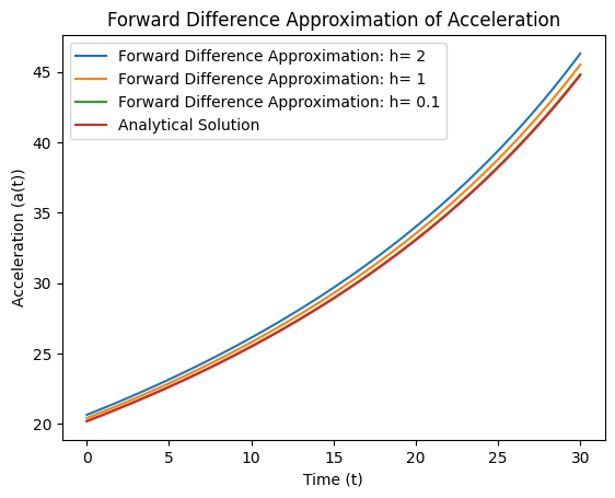
plt.plot(t, a_fd_h2, label='Forward Difference Approximation: h= 2')
plt.plot(t, a_fd_h1, label='Forward Difference Approximation: h= 1')
plt.plot(t, a_fd_h0p1, label='Forward Difference Approximation: h= 0.1')
plt.plot(t, a(t), label='Analytical Solution')
plt.xlabel('Time (t)')
plt.ylabel('Acceleration (a(t))')
plt.title('Forward Difference Approximation of Acceleration')
plt.legend()
plt.show()

Backward difference

By contrast, the backward difference steps backwards. Consider replacing \(h\) with \(-h\),

\[ f(x-h) = f(x) - f'(x) h + O(h^2)\]

and solve for:

\[f'(x) = \frac{f(x)- f(x-h)}{h} + O(h^2) \]

def backward_difference(f, x, h):
  return (f(x)- f(x - h)) / h

a_bd_h2 = backward_difference(v, t, h = 2)
a_bd_h1 = backward_difference(v, t, h = 1)
a_bd_h0p1 = backward_difference(v, t, h = 0.1)

# Plotting the results
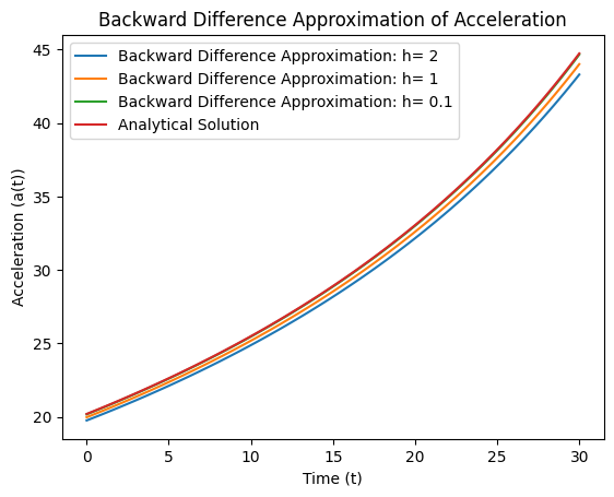
plt.plot(t, a_bd_h2, label='Backward Difference Approximation: h= 2')
plt.plot(t, a_bd_h1, label='Backward Difference Approximation: h= 1')
plt.plot(t, a_bd_h0p1, label='Backward Difference Approximation: h= 0.1')
plt.plot(t, a(t), label='Analytical Solution')
plt.xlabel('Time (t)')
plt.ylabel('Acceleration (a(t))')
plt.title('Backward Difference Approximation of Acceleration')
plt.legend()
plt.show()

Note that the approximations are approaching the analytic solution from the other direction.

Can we combine forward and backward differences to get a better result?

Central difference

Let’s examine the forward and backward expansions:

\[\begin{split} \begin{align} f(x+h) &= f(x) + f'(x) h + f''(x) \frac{h^2}{2} + f'''(x)\frac{h^3}{6} + O(h^4) \\ f(x-h) &= f(x) - f'(x) h + f''(x) \frac{h^2}{2} - f'''(x)\frac{h^3}{6} + O(h^4) \\ \end{align} \end{split}\]

and subtract them: $\( f(x+h)-f(x-h) = 2 f'(x) h + f''' \frac{h^3}{3} + O(h^5) \)\( Note that the even powers of \)h$ cancel!

Rearranging this equation leads to the central difference formula: $\( f'(x) = \frac{f(x+h)-f(x-h)}{2h} + O(h^2) \)$

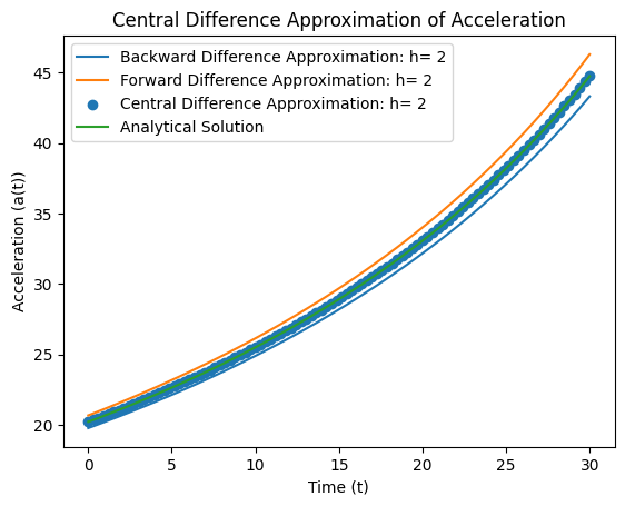
which is second order accurate in \(h\) since the next correction is \(h^2\)!

def central_difference(f, x, h):
  return (f(x+h)- f(x - h)) / (2*h)

a_cd_h1 = central_difference(v, t, h = 1)
a_cd_h2 = central_difference(v, t, h = 2)

# Plotting the results
plt.plot(t, a_bd_h2, label='Backward Difference Approximation: h= 2')
plt.plot(t, a_fd_h2, label='Forward Difference Approximation: h= 2')
plt.scatter(t, a_cd_h2, label='Central Difference Approximation: h= 2')
plt.plot(t, a(t), label='Analytical Solution')
plt.xlabel('Time (t)')
plt.ylabel('Acceleration (a(t))')
plt.title('Central Difference Approximation of Acceleration')
plt.legend()
plt.show()

Comparison

Lets comare the error in forward, backward and central difference for \(h=2\):

np.stack([a_fd_h2-a(t), a_bd_h2-a(t), a_cd_h2-a(t)]).T[1:5,:]

array([[ 0.46345415, -0.44519649,  0.00912883],
       [ 0.46776   , -0.44924984,  0.00925508],
       [ 0.47212613, -0.4533588 ,  0.00938366],
       [ 0.47655369, -0.4575244 ,  0.00951465]])

Let’s see how it scales with decreasing step size between \(h=2\) and \(h' = 1\):

np.stack([a_fd_h2-a(t), a_fd_h1-a(t)]).T[1:5,:]

array([[0.46345415, 0.22936654],
       [0.46776   , 0.23148645],
       [0.47212613, 0.23363589],
       [0.47655369, 0.2358154 ]])

np.stack([a_bd_h2-a(t), a_bd_h1-a(t)]).T[1:5,:]

array([[-0.44519649, -0.22480399],
       [-0.44924984, -0.22686082],
       [-0.4533588 , -0.22894601],
       [-0.4575244 , -0.23106008]])

Note the error roughly cuts in half; \(Error \sim \frac{h}{h'}\). Now take a look at the central difference:

np.stack([a_cd_h2-a(t), a_cd_h1-a(t)]).T[1:5,:]

array([[0.00912883, 0.00228127],
       [0.00925508, 0.00231281],
       [0.00938366, 0.00234494],
       [0.00951465, 0.00237766]])

See how it reduces by a factor of 4: \(Error \sim \bigg[\frac{h}{h'}\bigg]^2\)

The central difference algorithm:

• finds a more accurate solution in the same number of function calls.

• becomes more accurate with step size quadratically.

• requires information both before and after the point (which can be a problem at boundaries).