Matrix types#
LU decomposition has useful properties depending on the types of matricies involved.
Symbol |
Matrix Type |
Example 2x2 |
Interesting Properties |
|---|---|---|---|
0 |
Zero |
\(\begin{bmatrix} 0 & 0 \\ 0 & 0 \end{bmatrix}\) |
A-A = 0 |
I |
Identity |
\(\begin{bmatrix} 1 & 0 \\ 0 & 1 \end{bmatrix}\) |
A I = A |
D |
Diagonal |
\(\begin{bmatrix} d_1 & 0 \\ 0 & d_2 \end{bmatrix}\) |
\(D^{-1}\) = \(\begin{bmatrix} d_1^{-1} & 0 \\ 0 & d_2^{-1} \end{bmatrix}\) |
U |
Upper Triangular |
\(\begin{bmatrix} 1 & 2 \\ 0 & 4 \end{bmatrix}\) |
\(U^{-1}\) is another upper triangular matrix |
L |
Lower Triangular |
\(\begin{bmatrix} 5 & 0 \\ -1 & 2 \end{bmatrix}\) |
\(L^{-1}\) is another lower triangular matrix |
P |
Permutation |
\(\begin{bmatrix} 0 & 1 \\ 1 & 0 \end{bmatrix}\) |
Its transpose is its inverse (\(P^T = P^{-1}\)) |
S |
Symmetric |
\(\begin{bmatrix} 1 & 3 \\ 3 & -4 \end{bmatrix}\) |
Equal to its transpose (\(S = S^T\)). |
SPD |
Symmetric positive definite |
\(\begin{bmatrix} 1 & 3 \\ 3 & 4 \end{bmatrix}\) |
\(x^T [SPD] x >0\) - think of a quadratic |
Sparse matricies and sparsity patterns#
Sparsity refers to the fraction of non-zero elements in a matrix. Sparse matricies have a significant fraction of 0 elements, which can drastically reduce storage and computational requirements.
Storage: Typically one (conceptually) stores a matrix as a 2D array. With significant sparsity, one can instead store only non-zero entries. There is a trade-off here between access / modification and memory efficiency.
Computation: (Fill-in) Fill-in is the phenomena where, during computation, zeros become non-zeros. This disrupts the sparsity pattern and the benefits that accompany it, and is hence something to be avoided.
Sparsity patterns and matrix#
Sparsity patterns are condensly viewed as monochrome matricies filled in according to 0 or non-zero.
Example: A sparsity pattern from a finite element problem in 2D.
We already have examples of sparse matricies with
diagonal
upper and lower triangular and have seen their importance in controlling complexity and roundoff error.
Banded matricies#
Banded matricies only have non-zero elements parallel to the diagonal. Sometimes they are described by the bandwidth, the number of parallel bands.
Tridiagonal (bandwidth 3)#
# prompt: give me a tridiagonal matrix of dimension 10 and view its sparsity pattern with spy

import numpy as np
import matplotlib.pyplot as plt

# Create a tridiagonal matrix of dimension 10
n = 10
T = np.zeros((n, n))
np.fill_diagonal(T, 2)  # Main diagonal
np.fill_diagonal(T[1:], -1)  # Lower diagonal
np.fill_diagonal(T[:, 1:], -1)  # Upper diagonal

print(T)

# View the sparsity pattern
plt.spy(T)
plt.show()
[[ 2. -1.  0.  0.  0.  0.  0.  0.  0.  0.]
 [-1.  2. -1.  0.  0.  0.  0.  0.  0.  0.]
 [ 0. -1.  2. -1.  0.  0.  0.  0.  0.  0.]
 [ 0.  0. -1.  2. -1.  0.  0.  0.  0.  0.]
 [ 0.  0.  0. -1.  2. -1.  0.  0.  0.  0.]
 [ 0.  0.  0.  0. -1.  2. -1.  0.  0.  0.]
 [ 0.  0.  0.  0.  0. -1.  2. -1.  0.  0.]
 [ 0.  0.  0.  0.  0.  0. -1.  2. -1.  0.]
 [ 0.  0.  0.  0.  0.  0.  0. -1.  2. -1.]
 [ 0.  0.  0.  0.  0.  0.  0.  0. -1.  2.]]
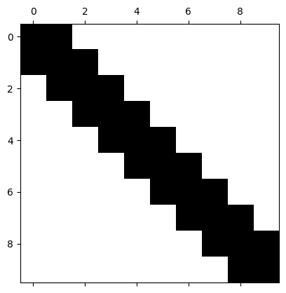
Pentadiagonal (bandwidth 5)#
# prompt: give me a pentadiagonal matrix of dimension 10 and view its sparsity pattern with spy

import numpy as np
import matplotlib.pyplot as plt

# Create a pentadiagonal matrix of dimension 10
n = 10
A = np.zeros((n, n))
np.fill_diagonal(A, 2)  # Main diagonal
np.fill_diagonal(A[1:], -1)  # Upper diagonal
np.fill_diagonal(A[:, 1:], -1)  # Lower diagonal
np.fill_diagonal(A[2:], -1)  # Second upper diagonal
np.fill_diagonal(A[:, 2:], -1)  # Second lower diagonal

print(A)

# View the sparsity pattern
plt.spy(A)
plt.show()
[[ 2. -1. -1.  0.  0.  0.  0.  0.  0.  0.]
 [-1.  2. -1. -1.  0.  0.  0.  0.  0.  0.]
 [-1. -1.  2. -1. -1.  0.  0.  0.  0.  0.]
 [ 0. -1. -1.  2. -1. -1.  0.  0.  0.  0.]
 [ 0.  0. -1. -1.  2. -1. -1.  0.  0.  0.]
 [ 0.  0.  0. -1. -1.  2. -1. -1.  0.  0.]
 [ 0.  0.  0.  0. -1. -1.  2. -1. -1.  0.]
 [ 0.  0.  0.  0.  0. -1. -1.  2. -1. -1.]
 [ 0.  0.  0.  0.  0.  0. -1. -1.  2. -1.]
 [ 0.  0.  0.  0.  0.  0.  0. -1. -1.  2.]]
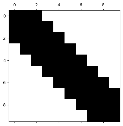
One can imagine the benefit of storing such a matrix
General banded matrix#
import numpy as np
import matplotlib.pyplot as plt

# Create a pentadiagonal matrix of dimension 10
n = 10
A = np.zeros((n, n))
np.fill_diagonal(A, 2)  # Main diagonal
np.fill_diagonal(A[1:], -1)  # Upper diagonal
np.fill_diagonal(A[:, 1:], -1)  # Lower diagonal
np.fill_diagonal(A[4:], -2)  # Second upper diagonal
np.fill_diagonal(A[:, 4:], -1)  # Second lower diagonal

print(A)

# View the sparsity pattern
plt.spy(A)
plt.show()
[[ 2. -1.  0.  0. -1.  0.  0.  0.  0.  0.]
 [-1.  2. -1.  0.  0. -1.  0.  0.  0.  0.]
 [ 0. -1.  2. -1.  0.  0. -1.  0.  0.  0.]
 [ 0.  0. -1.  2. -1.  0.  0. -1.  0.  0.]
 [-2.  0.  0. -1.  2. -1.  0.  0. -1.  0.]
 [ 0. -2.  0.  0. -1.  2. -1.  0.  0. -1.]
 [ 0.  0. -2.  0.  0. -1.  2. -1.  0.  0.]
 [ 0.  0.  0. -2.  0.  0. -1.  2. -1.  0.]
 [ 0.  0.  0.  0. -2.  0.  0. -1.  2. -1.]
 [ 0.  0.  0.  0.  0. -2.  0.  0. -1.  2.]]
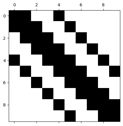
Block matricies#
Block matricies can be partitioned:
with
and
The inverse can be formed:
This is a substantial savings since the cost of each block scales exponentially!
Sometimes we get lucky and one of the blocks is \(0\) or \(I\) which is a HUGE benefit!
If the blocks are each \(n \times n\), \(M\) is \(2n \times 2n\) and takes \(O((2n)^3)\) to solve. But if we partition into blocks, the inverse can be formed in 2 separate \(O(n^3)\) (plus matrix multiplications).
This situation arises commonly in multiphysics applications, with two fields (e.g.: T and c). The blocks are then defined corresponding to the unknown vectors for each field.
Certaint types of physics is solved more efficiently with certain solvers. This decomposition, sometimes called operator splitting or segregated solving allows each variable (block) to be treated optimally and inverse of the full system assembled.
In contrast, solving the matrix as a whole is called a monolithic solution.
Block diagonal#
Taking \(B=C=0\) in the above we can see the inverse of a block diagonal matrix is simply the diagonal assembly of the inverse of its blocks:
Matrix decompositions#
We can now summarize some decompositions:
Matrix equation |
Operation count |
|---|---|
\(A = LU\) |
\(n^3/3\) |
\(S = L D L^T\) |
\(n^3/6\) |
\(SPD = L L^T\) |
\(n^3/6\) + n |
The later two are called Choleski decomposition and take advantage of matrix symmetry for efficiency.
Since in general
\(A^{-1} = [LU]^{-1} = U^{-1} L^{-1}\)
it would be tempting to calculate and store \(A^{-1}\) instead of \(L\) and \(U\), but this is not preferred due to the impact on sparsity, in addition to round-off error \(\propto |A|^{-1}\).
##Decompositions of certain matricies
Inverse of a triangular matrix is triangular#
# prompt: show the inverse of an upper triangular matrix with numpy

import numpy as np
# Create an upper triangular matrix
A = np.array([[1, 2, 3],
              [0, 4, 5],
              [0, 0, 6]])

# Calculate the inverse
A_inv = np.linalg.inv(A)

print("Upper triangular matrix:\n", A)
print("\nInverse of the upper triangular matrix:\n", A_inv)
Upper triangular matrix:
 [[1 2 3]
 [0 4 5]
 [0 0 6]]

Inverse of the upper triangular matrix:
 [[ 1.         -0.5        -0.08333333]
 [ 0.          0.25       -0.20833333]
 [ 0.          0.          0.16666667]]
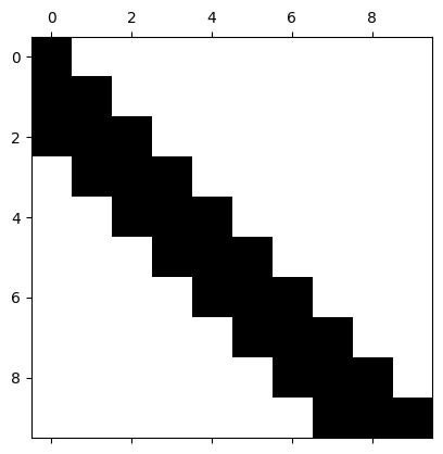
LU decomposition of a banded matrix is banded-triangular#
# prompt: Show that the choleski decomposition of a banded matrix is triangular-banded

import numpy as np
from scipy.linalg import cholesky
import matplotlib.pyplot as plt

# Create a pentadiagonal matrix of dimension 10
n = 10
A = np.zeros((n, n))
np.fill_diagonal(A, 2)  # Main diagonal
np.fill_diagonal(A[1:], 1)  # Upper diagonal
np.fill_diagonal(A[:, 1:], 1)  # Lower diagonal
np.fill_diagonal(A[2:], .1)  # Second upper diagonal
np.fill_diagonal(A[:, 2:], .1)  # Second lower diagonal

# Calculate the Cholesky decomposition
L = cholesky(A, lower=True)

print("Original matrix:\n", A)
print("\nCholesky decomposition (L):\n", np.around(L, decimals=2))

# View the sparsity pattern
plt.spy(L)
plt.show()
Original matrix:
 [[2.  1.  0.1 0.  0.  0.  0.  0.  0.  0. ]
 [1.  2.  1.  0.1 0.  0.  0.  0.  0.  0. ]
 [0.1 1.  2.  1.  0.1 0.  0.  0.  0.  0. ]
 [0.  0.1 1.  2.  1.  0.1 0.  0.  0.  0. ]
 [0.  0.  0.1 1.  2.  1.  0.1 0.  0.  0. ]
 [0.  0.  0.  0.1 1.  2.  1.  0.1 0.  0. ]
 [0.  0.  0.  0.  0.1 1.  2.  1.  0.1 0. ]
 [0.  0.  0.  0.  0.  0.1 1.  2.  1.  0.1]
 [0.  0.  0.  0.  0.  0.  0.1 1.  2.  1. ]
 [0.  0.  0.  0.  0.  0.  0.  0.1 1.  2. ]]

Cholesky decomposition (L):
 [[1.41 0.   0.   0.   0.   0.   0.   0.   0.   0.  ]
 [0.71 1.22 0.   0.   0.   0.   0.   0.   0.   0.  ]
 [0.07 0.78 1.18 0.   0.   0.   0.   0.   0.   0.  ]
 [0.   0.08 0.79 1.17 0.   0.   0.   0.   0.   0.  ]
 [0.   0.   0.08 0.8  1.16 0.   0.   0.   0.   0.  ]
 [0.   0.   0.   0.09 0.8  1.16 0.   0.   0.   0.  ]
 [0.   0.   0.   0.   0.09 0.8  1.16 0.   0.   0.  ]
 [0.   0.   0.   0.   0.   0.09 0.8  1.16 0.   0.  ]
 [0.   0.   0.   0.   0.   0.   0.09 0.8  1.16 0.  ]
 [0.   0.   0.   0.   0.   0.   0.   0.09 0.8  1.16]]
Inverse of a banded matrix is not banded (except diagonal)#
# prompt: show the inverse of a banded matrix in numpy

import numpy as np

# Create a tridiagonal matrix of dimension 10
n = 10
A = np.zeros((n, n))
np.fill_diagonal(A, 2)  # Main diagonal
np.fill_diagonal(A[1:], -1)  # Upper diagonal
np.fill_diagonal(A[:, 1:], -1)  # Lower diagonal

# Calculate the inverse
A_inv = np.linalg.inv(A)

print("Banded matrix:\n")
print(A)
plt.spy(A)
plt.show()
print("\nInverse of the banded matrix:\n")
print(A_inv)
plt.spy(A_inv)
plt.show()
Banded matrix:

[[ 2. -1.  0.  0.  0.  0.  0.  0.  0.  0.]
 [-1.  2. -1.  0.  0.  0.  0.  0.  0.  0.]
 [ 0. -1.  2. -1.  0.  0.  0.  0.  0.  0.]
 [ 0.  0. -1.  2. -1.  0.  0.  0.  0.  0.]
 [ 0.  0.  0. -1.  2. -1.  0.  0.  0.  0.]
 [ 0.  0.  0.  0. -1.  2. -1.  0.  0.  0.]
 [ 0.  0.  0.  0.  0. -1.  2. -1.  0.  0.]
 [ 0.  0.  0.  0.  0.  0. -1.  2. -1.  0.]
 [ 0.  0.  0.  0.  0.  0.  0. -1.  2. -1.]
 [ 0.  0.  0.  0.  0.  0.  0.  0. -1.  2.]]

Inverse of the banded matrix:

[[0.90909091 0.81818182 0.72727273 0.63636364 0.54545455 0.45454545
  0.36363636 0.27272727 0.18181818 0.09090909]
 [0.81818182 1.63636364 1.45454545 1.27272727 1.09090909 0.90909091
  0.72727273 0.54545455 0.36363636 0.18181818]
 [0.72727273 1.45454545 2.18181818 1.90909091 1.63636364 1.36363636
  1.09090909 0.81818182 0.54545455 0.27272727]
 [0.63636364 1.27272727 1.90909091 2.54545455 2.18181818 1.81818182
  1.45454545 1.09090909 0.72727273 0.36363636]
 [0.54545455 1.09090909 1.63636364 2.18181818 2.72727273 2.27272727
  1.81818182 1.36363636 0.90909091 0.45454545]
 [0.45454545 0.90909091 1.36363636 1.81818182 2.27272727 2.72727273
  2.18181818 1.63636364 1.09090909 0.54545455]
 [0.36363636 0.72727273 1.09090909 1.45454545 1.81818182 2.18181818
  2.54545455 1.90909091 1.27272727 0.63636364]
 [0.27272727 0.54545455 0.81818182 1.09090909 1.36363636 1.63636364
  1.90909091 2.18181818 1.45454545 0.72727273]
 [0.18181818 0.36363636 0.54545455 0.72727273 0.90909091 1.09090909
  1.27272727 1.45454545 1.63636364 0.81818182]
 [0.09090909 0.18181818 0.27272727 0.36363636 0.45454545 0.54545455
  0.63636364 0.72727273 0.81818182 0.90909091]]
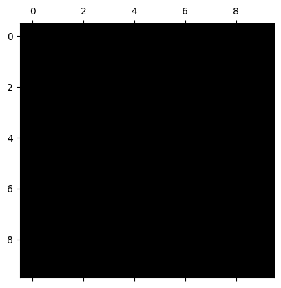
Yikes!!! :-(
#Package implementations
Numpy and Scipy linear solvers both do (P)LU decomposition and then solution. In general they can be accessed through:
numpy.linalg.solve(A,b)
and
scipy.linalg.solve(A,b)
Examining the options of scipy show that you can choose to:
specify the matrix type
overwrite the original matricies (which may boost efficiency)
The advent of distributed computing (HPCs) motivated new algorithms that are better suited to large, sparse, systems (You will run in to these names in the future!)
PARADISO (PARallel Direct SOlver)
SuperLU (Supernodal LU)
UMFPACK (Unsymmetric-pattern MultiFrontal method)
MUMPS (Multifrontal Massively Parallel Sparse Direct Solver)
# prompt: use numpy to solve a linear system then repeat with scipy

import numpy as np
from scipy.linalg import solve

# Define the coefficient matrix A
A = np.array([[2, -1, 0],
              [-1, 2, -1],
              [0, -1, 2]])

# Define the right-hand side vector b
b = np.array([1, 2, 3])

# Solve the linear system using numpy.linalg.solve
x_numpy = np.linalg.solve(A, b)
print("Solution using numpy.linalg.solve:\n", x_numpy)

# Solve the linear system using scipy.linalg.solve
x_scipy = solve(A, b)
print("\nSolution using scipy.linalg.solve:\n", x_scipy)
Solution using numpy.linalg.solve:
 [2.5 4.  3.5]

Solution using scipy.linalg.solve:
 [2.5 4.  3.5]
# prompt: solve a 200x200 sparse system with sparse solvers then again  with a dense solver

import numpy as np
from scipy.sparse import diags
from scipy.sparse.linalg import spsolve
from scipy.linalg import solve

# Generate a random sparse matrix
n = 200

main_diag = np.full(n, 2)
upper_diag = np.full(n - 1, -1)
lower_diag = np.full(n - 1, -1)
A_sparse = diags([lower_diag, main_diag, upper_diag], offsets=[-1, 0, 1], format='csr')


# row_ind = np.arange(n)
# col_ind = np.arange(n)
# data = np.random.rand(n)
# A_sparse = csr_matrix((data, (row_ind, col_ind)), shape=(n, n))

# Generate a random right-hand side vector
b = np.random.rand(n)

# Solve the sparse system
%timeit x_sparse = spsolve(A_sparse, b)
#print("Solution using sparse solver:\n", x_sparse, "\n")

# Convert the sparse matrix to a dense matrix
A_dense = A_sparse.toarray()

# Solve the dense system

%timeit x_dense = solve(A_dense, b)
#print("Solution using dense solver:\n", x_dense)
307 µs ± 142 µs per loop (mean ± std. dev. of 7 runs, 1000 loops each)
1.29 ms ± 101 µs per loop (mean ± std. dev. of 7 runs, 100 loops each)

