Solvability#
You are organizing a fundraising event and need to buy chairs and tables. Chairs cost $20 each and tables cost $50 each. You have a budget of $700 and need a total of 20 pieces of furniture (chairs and tables combined). How many chairs and tables should you buy?
import sys
sys.path.append('../Tools')
from module import LinearSystemSolverPlotly
['LinearSystemSolverNotebook', '__builtins__', '__cached__', '__doc__', '__file__', '__loader__', '__name__', '__package__', '__spec__', 'clear_output', 'display', 'np', 'plt', 'widgets']
A system with one solution#
Let \(c\) and \(t\) be the number of chairs and tables respectively. The budget and pieces equations are,
(1) \(20 c + 50 t = 700\)
(2) \( c+t = 20\)
There are a few ways to solve these equations.
Solve graphically#
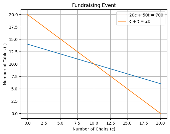
Since these are lines, let’s plot them!
# prompt: Plot the two lines with a grid

import matplotlib.pyplot as plt
import numpy as np
# Define the x values
x = np.linspace(0, 20, 100)

# Calculate the y values for the first equation (20c + 50t = 700)
y1 = (700 - 20 * x) / 50

# Calculate the y values for the second equation (c + t = 20)
y2 = 20 - x

# Plot the lines
plt.plot(x, y1, label='20c + 50t = 700')
plt.plot(x, y2, label='c + t = 20')

# Add labels and title
plt.xlabel('Number of Chairs (c)')
plt.ylabel('Number of Tables (t)')
plt.title('Fundraising Event')

# Add a grid
plt.grid(True)

# Add a legend
plt.legend()

# Display the plot
plt.show()

The point where the lines intersect satisfy both equations and is therefore a solution. Since lines only cross once, it is the unique solution.
Solve through elimination#
Multiply the second equation, (2), by \(20\):
(3) \(20c+20t = 400\).
Subtract (3) from (1) and simplify:
\(30t = 300\)
\(t=10\)
Substitute answer into (2):
\(c = 10\)
Matrix formulation and solution#
Writting these as a matrix equation becomes:
\(\begin{pmatrix} 20 & 50 \\ 1 &1 \end{pmatrix} \begin{pmatrix} c \\ t \end{pmatrix} = \begin{pmatrix} 700 \\ 20 \end{pmatrix}\)
or in standard form,
\(A x = b\)
with \(A = \begin{pmatrix} 20 & 50 \\ 1 &1 \end{pmatrix}\)
\(x = \begin{pmatrix} c \\ t \end{pmatrix}\)
\(b = \begin{pmatrix} 700 \\ 20 \end{pmatrix}\)
Let’s find \(A^{-1}\) such that \(x = A^{-1}b\). For a square matrix of dimensions 2x2:
\(\begin{pmatrix} a & b \\ c & d \end{pmatrix}^{-1} = \frac{1}{|A|} \begin{pmatrix} d & -b \\ -c & a \end{pmatrix}\)
where \(|A| = ad-bc\) is the determinant.
The prefactor of \(\frac{1}{|A|}\) is systemic to inversion. In general, \(A^{-1} = \frac{1}{|A|} adj(A)\) for square matricies of any dimension.
For our case,
\(|A| = -30\), and
\(A^{-1} = \frac{1}{-30} \begin{pmatrix} 1 & -50 \\ -1 & 20 \end{pmatrix}\)
thus, \(A^{-1} b\):
\(x = \begin{pmatrix} 10 \\ 10 \end{pmatrix} \)
Infinite solutions#
Lets tweak our problem and see what happens.
There is now a discount on tables down to $20 each. The customer heard about it and cut your budget to $400.
The problem is now:
\(20 c + 20 t = 400\)
\( c+t = 20\)
Graphically#
# prompt: Plot the two lines with a grid making the first line thicker

import matplotlib.pyplot as plt
import numpy as np
# Define the x values
x = np.linspace(0, 20, 100)

# Calculate the y values for the first equation (20c + 20t = 400)
y1 = (400 - 20 * x) / 20

# Calculate the y values for the second equation (c + t = 20)
y2 = 20 - x

# Plot the lines
plt.plot(x, y1, label='20c + 20t = 400', linewidth=3)  # Make the first line thicker
plt.plot(x, y2, label='c + t = 20')

# Add labels and title
plt.xlabel('Number of Chairs (c)')
plt.ylabel('Number of Tables (t)')
plt.title('Fundraising Event (Revised)')

# Add a grid
plt.grid(True)

# Add a legend
plt.legend()

# Display the plot
plt.show()

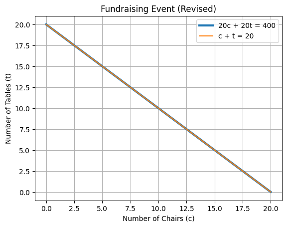
The lines overlap! What does this mean?
Elimination#
Multiple second row by 20:
\(20c+20t = 400\)
subtracting the first we get,
\(0=0\)
:-(
Solve the second equation to find \(c = 20/t\)
and that’s it! For all \(t\) there is a \(c\) that is a solution!
The matrix equation#
\(|A| = ad−bc = 0\)
What does this mean for the inverse \(A^{-1}\)?
No solutions#
WOOPS! The customer meant to say $500; no more, no less!
The problem is now
\(20 c + 20 t = 500\)
\( c+t = 20\)
Graphically#
# prompt: Graph it again please!

import matplotlib.pyplot as plt
import numpy as np
# Define the x values
x = np.linspace(0, 20, 100)

# Calculate the y values for the first equation (20c + 20t = 500)
y1 = (500 - 20 * x) / 20

# Calculate the y values for the second equation (c + t = 20)
y2 = 20 - x

# Plot the lines
plt.plot(x, y1, label='20c + 20t = 500', linewidth=3)  # Make the first line thicker
plt.plot(x, y2, label='c + t = 20')

# Add labels and title
plt.xlabel('Number of Chairs (c)')
plt.ylabel('Number of Tables (t)')
plt.title('Fundraising Event (Revised Again)')

# Add a grid
plt.grid(True)

# Add a legend
plt.legend()

# Display the plot
plt.show()

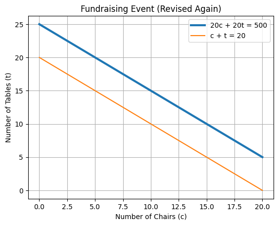
Now they are parralel! What does THIS mean?
Elimination#
The second row multiplied by 20 is still \(20c+20t = 400\) (!!). Now subtracting the first becomes:
\(20c + 20t = 500\)
-\(20c - 20t = -400\)
\(-----------------\)
\(0+0=100\)
… >:-(
And the matrix equation?#
Unchanged since only \(b\) has change!
(What does this tell you?!?)
Putting it together#
Linear equations (in 2 unkowns) are lines in 2D. The solution is the intersection of those lines. 2 Lines can intersect either
in one place (the first example)
everywhere (the second example)
nowhere (the third example)
For 2 and 3, these lines are parallel, i.e. you can slide one to lie ontop of the other.Such lines are called linearly dependent.
Example 1 has linear independent equations which intersect in one place and can be solved.
Scenarios 1 and 2 are called a consistent linear system since an answer can be obtained. Scenario 3 is inconsistent since there is no solution.
The matrix interpretation#
The coefficient matrix \(A\) depends on the nature of the lines, not the constant. When
\(|A| = 0\),
The matrix \(A\) is termed singular. The lines are parallel, which means the equations / rows in \(A\) and linear dependant and you will not be able to solve for a unique \(x\).
This is true regardless of the values of \(b\)!


