Radial Basis Functions

Radial basis functions are an n-dimensional interpolation technique that doesn’t rely on polynomials. Rather, we define a radial basis function, called a kernel, applied to each data point:

\[\varphi_i(||x-x_i||)\]

Commonly, we say \(\varphi_i(x=x_i)\equiv 1\).

The kernel only depends on the Euclidian distance between the associated data point, \(x_i\) and the evaluation point \(x\) (and are therefore radial).

The interpolation function \(y(x)\) is the weighted sum of the \(N\) kernels:

\[y(x) = \sum_i^N \omega_i \varphi_i(||x-x_i||)\]

To determine the weights \(w_i\), we use the data points we have. Consider the \(i\)’th datapoints,

\[y(x_i) = \sum_j^N \omega_j \varphi_j(||x-x_j||)=y_i\]

and applied to all N data points generates a linear system:

\[\begin{split} \begin{bmatrix} \phi(\|x_1 - x_1\|) & \phi(\|x_1 - x_2\|) & \cdots & \phi(\|x_1 - x_n\|) \\ \phi(\|x_2 - x_1\|) & \phi(\|x_2 - x_2\|) & \cdots & \phi(\|x_2 - x_n\|) \\ \vdots & \vdots & \ddots & \vdots \\ \phi(\|x_n - x_1\|) & \phi(\|x_n - x_2\|) & \cdots & \phi(\|x_n - x_n\|) \end{bmatrix} \begin{bmatrix} \omega_1 \\ \omega_2 \\ \vdots \\ \omega_n \end{bmatrix} = \begin{bmatrix} y_1 \\ y_2 \\ \vdots \\ y_n \end{bmatrix} \end{split}\]

which we know how to solve!

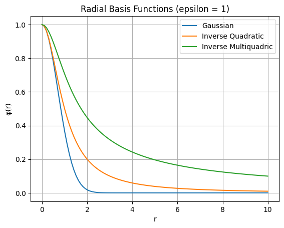
Kernels are defined with \(r = \| x-x_i\|\) and a tuning parameter \(\epsilon\). Some common simple kernels are:

Kernel	Formula
Gaussian	\(e^{-\epsilon^2 r^2}\)
Inverse quadratic	\(\frac{1}{1+[\epsilon r ]^2}\)
Inverse multiquadric	\(\frac{1}{\sqrt{1+[\epsilon r ]^2}}\)

Determination of optimal \(\epsilon\) is a nuanced question, but a good rule of thumb is to use the average distance between samples.

\(\epsilon = avg \|x_i-x_j\|\)

Let’s see the kernels:

# prompt: Plot the above radial basis functions for epsilon = 1

import numpy as np
import matplotlib.pyplot as plt

# Define the radial basis functions
def gaussian(r, epsilon):
  return np.exp(-(epsilon * r)**2)

def inverse_quadratic(r, epsilon):
  return 1 / (1 + (epsilon * r)**2)

def inverse_multiquadric(r, epsilon):
  return 1 / np.sqrt(1 + (epsilon * r)**2)

epsilon = 1

# Create a range of r values
r_values = np.linspace(0, 10, 100)

# Calculate the function values for each kernel
gaussian_values = gaussian(r_values, epsilon)
inverse_quadratic_values = inverse_quadratic(r_values, epsilon)
inverse_multiquadric_values = inverse_multiquadric(r_values, epsilon)

# Plot the radial basis functions
plt.plot(r_values, gaussian_values, label='Gaussian')
plt.plot(r_values, inverse_quadratic_values, label='Inverse Quadratic')
plt.plot(r_values, inverse_multiquadric_values, label='Inverse Multiquadric')

plt.xlabel('r')
plt.ylabel('φ(r)')
plt.title('Radial Basis Functions (epsilon = 1)')
plt.legend()
plt.grid(True)
plt.show()

In general, \(\varphi_i(r=0)\) is not necessarily \(1\), and \(\varphi(r \rightarrow \infty) \ne 0\), but this requires one more key factor to implement robustly.

Example - Our Toy problem from last lecture (Gaussian sampled at 10 points, equally spaced)

#Sampled gaussian

import numpy as np
import matplotlib.pyplot as plt

# Define the function
def f(x):
  return np.exp(-(x/2)**2)

def gaussian(r, epsilon):
  return np.exp(-(epsilon * r)**2)

# Create x values for plotting
x_toy = np.linspace(-6, 6, 100)
y_toy = f(x_toy)

# Sample 11 times at 1-interval intervals
x_d = np.arange(-5, 6, 1)
y_d = f(x_d)

# prompt: Construct gaussian radial basis functions and fit to y_d and x_d

import matplotlib.pyplot as plt
import numpy as np
# Create a matrix of the radial basis functions
phi_matrix = np.zeros((len(x_d), len(x_d)))

epsilon = 1

for i in range(len(x_d)):
  for j in range(len(x_d)):
    phi_matrix[i, j] = gaussian(np.abs(x_d[i] - x_d[j]), epsilon)

#~~ How do we solve for w_i?
# Take a look at the matrix!



# #~~ Answer
# np.set_printoptions(precision=2, suppress=True)
# print(phi_matrix)
# weights = np.linalg.solve(phi_matrix, y_d)
# #~~

# Define the interpolation function
def interpolation_function(x, weights, x_d, epsilon):
  y = 0
  for i in range(len(x_d)):
    y += weights[i] * gaussian(np.abs(x - x_d[i]), epsilon)
  return y

# Interpolate y_fit
y_fit = [interpolation_function(x, weights, x_d, epsilon) for x in x_toy]

# Plot the results
plt.plot(x_toy, y_toy, label='Original Function')
plt.scatter(x_d, y_d, color='red', label='Data Points')
plt.plot(x_toy, y_fit, label='Interpolation', linestyle='--')

plt.xlabel('x')
plt.ylabel('y')
plt.title('Radial Basis Function Interpolation (Gaussian Kernel)')
plt.legend()
plt.grid(True)
plt.show()

---------------------------------------------------------------------------
NameError                                 Traceback (most recent call last)
Cell In[3], line 33
     30   return y
     32 # Interpolate y_fit
---> 33 y_fit = [interpolation_function(x, weights, x_d, epsilon) for x in x_toy]
     35 # Plot the results
     36 plt.plot(x_toy, y_toy, label='Original Function')

Cell In[3], line 33, in <listcomp>(.0)
     30   return y
     32 # Interpolate y_fit
---> 33 y_fit = [interpolation_function(x, weights, x_d, epsilon) for x in x_toy]
     35 # Plot the results
     36 plt.plot(x_toy, y_toy, label='Original Function')

NameError: name 'weights' is not defined

Note this is a great result, but it works because the true function tends to zero outside of the data samples.

Example - 2D gaussian

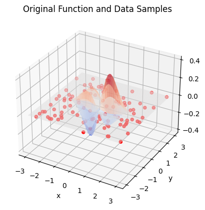
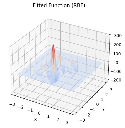
# prompt: Generate a function exp(-x^2-7*y^2)*sin(x)*cos(8y), sample 100 times and fit using gaussian radial basis functions as done above. Plot the original function with the data samples, then the fit.

import numpy as np
import matplotlib.pyplot as plt
from mpl_toolkits.mplot3d import Axes3D
from matplotlib import cm

# Define the function
def f(x, y):
  return np.exp(-x**2 - 7*y**2) * np.sin(x) * np.cos(8*y)

# Create a grid of x and y values
x = np.linspace(-3, 3, 100)
y = np.linspace(-3, 3, 100)
X, Y = np.meshgrid(x, y)
Z = f(X, Y)

# Sample 100 times
num_samples = 100
x_samples = np.random.uniform(-3, 3, num_samples)
y_samples = np.random.uniform(-3, 3, num_samples)
z_samples = f(x_samples, y_samples)

# Plot the original function and data samples
fig = plt.figure()
ax = fig.add_subplot(111, projection='3d')
ax.plot_surface(X, Y, Z, cmap=cm.coolwarm, alpha=0.5)
ax.scatter(x_samples, y_samples, z_samples, color='red', marker='o', s=20)
ax.set_xlabel('x')
ax.set_ylabel('y')
ax.set_zlabel('z')
ax.set_title('Original Function and Data Samples')
plt.show()



# Define the radial basis function (Gaussian)
def gaussian_2d(x1, y1, x2, y2, epsilon):
    r = np.sqrt((x1 - x2)**2 + (y1 - y2)**2)
    return np.exp(-(epsilon * r)**2)

def phi_matrix_2d(x_samples, y_samples, epsilon):
    num_samples = len(x_samples)
    phi_matrix = np.zeros((num_samples, num_samples))
    for i in range(num_samples):
        for j in range(num_samples):
            phi_matrix[i, j] = gaussian_2d(x_samples[i], y_samples[i], x_samples[j], y_samples[j], epsilon)
    return phi_matrix

phi_matrix = phi_matrix_2d(x_samples, y_samples, epsilon = 1)

# #~~ Examine the condition number of the matrix before inverting it.
# print('The matrix condition number is, ', np.linalg.cond(phi_matrix))
# distances = []
# for i in range(num_samples):
#   for j in range(i + 1, num_samples):
#     distance = np.sqrt((x_samples[i] - x_samples[j])**2 + (y_samples[i] - y_samples[j])**2)
#     distances.append(distance)
# average_distance = np.mean(distances)
# eps = average_distance
# phi_matrix = phi_matrix_2d(x_samples, y_samples, epsilon= eps)
# print('The matrix condition number is, ', np.linalg.cond(phi_matrix))
# #~~~

# Calculate the weights
weights = np.linalg.solve(phi_matrix, z_samples)



# Define the interpolation function
def interpolation_function_2d(x, y, weights, x_samples, y_samples, epsilon):
    z = 0
    for i in range(num_samples):
        z += weights[i] * gaussian_2d(x, y, x_samples[i], y_samples[i], epsilon)
    return z

# Interpolate Z_fit
Z_fit = np.zeros((100, 100))
for i in range(100):
    for j in range(100):
        Z_fit[i, j] = interpolation_function_2d(x[i], y[j], weights, x_samples, y_samples, epsilon=3)

# Plot the fitted function
fig = plt.figure()
ax = fig.add_subplot(111, projection='3d')
ax.plot_surface(X, Y, Z_fit, cmap=cm.coolwarm, alpha=0.5)
ax.set_xlabel('x')
ax.set_ylabel('y')
ax.set_zlabel('z')
ax.set_title('Fitted Function (RBF)')
plt.show()