Optimization

Optimzation asks us to:

Find \(x\) that minimizes \(f(\vec{x}\)) subject to \(\vec{g}(\vec{x}) = 0\) and \(\vec{h}(\vec{x})\ge 0\)

• \(f\) is the objective function and typically a scalar

• \(\vec{g}(\vec{x})\) is a list of equality constraints

• \(\vec{h}(\vec{x})\) is a list of inequality constraints

• Maximization for \(f\) is mearly minimization of \(-f\).

• Optimization differs from root finding in the constraints and smoothness of \(f\).

We saw with root finding that using gradient information to help search algorithms has important benefits. That remains true in optimization, but since they are often high dimensional (\(\vec{x}\) is a large vector), and \(f\) is not necessarily well behaved, great value is placed on methods that do not require (direct) gradient / Hessian calculations.

Local vs Global minima

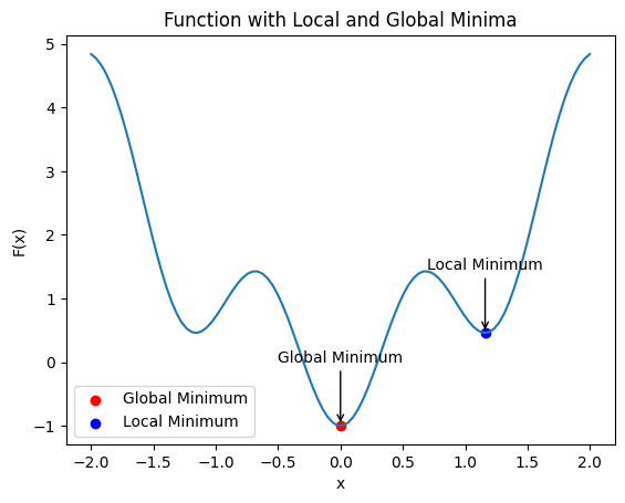
Even in 1D, optimization is confounded by local minimima. The lowest of the local minima is the global minimum.

There is no good way to ensure a local minimia is a global one without calculating and comparing them all!

There are lots of algorithms that attempt to find the global minimum. They either:

• launch multiple minimizers over the range of arguments

• typically involve preturbing good solutions in an attempt to escape from local minima basins.

Interestingly, many of these methods are modelled after nature! (Why?)

• Genetic algorithms - mutations, cross-overs, selection)

• Simulated annealing - metalurgical process that accepts worse solutions)

• Partical swarm - Mimics swarming behaviour to track multiple solutions

• Amoeba search (which we will talk about)

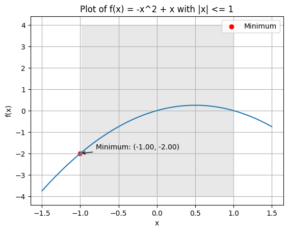
Introduction of constraints can further complicate things since sometimes the minimima is at a bound!

Example: local and global minimima

Minimize \(f = x^2 - cos(5 x)\)

# prompt: Draw a function with a clear local and global minima, labelled

import matplotlib.pyplot as plt
import numpy as np
import scipy as sp

x = np.linspace(-2, 2, 100)
f = lambda x: x**2 + -np.cos(5 * x)
y = f(x)

plt.plot(x, y)
plt.xlabel("x")
plt.ylabel("F(x)")
plt.title("Function with Local and Global Minima")

# Annotate the global minimum
plt.scatter(0, np.min(y), color='red', label='Global Minimum')
plt.annotate('Global Minimum', xy=(0, np.min(y)), xytext=(0, np.min(y) + 1), ha='center', arrowprops=dict(arrowstyle='->'))

# Annotate a local minimum (approximately)
opt =  sp.optimize.minimize(f,1)
local_min_x = opt.x
local_min_y = opt.fun
plt.scatter(local_min_x, local_min_y, color='blue', label='Local Minimum')
plt.annotate('Local Minimum', xy=(local_min_x, local_min_y), xytext=(local_min_x, local_min_y + 1), ha='center', arrowprops=dict(arrowstyle='->'))

plt.legend()
plt.show()

Example: Eggholder surfaces

Minimize \(y \cdot sin(\sqrt{\|x + y\|}) + x \cdot sin(\sqrt{\|x - y\|})\)

11# prompt: Draw a 2D eggholder surface using plotly

import plotly.graph_objects as go
import numpy as np

def eggholder(x, y):
  return y* np.sin(np.sqrt(abs(x + y ))) + x * np.sin(np.sqrt(abs(x - y)))


x = np.linspace(-512, 512, 100)
y = np.linspace(-512, 512, 100)
X, Y = np.meshgrid(x, y)
Z = eggholder(X, Y)/10

fig = go.Figure(data=[go.Surface(z=Z, x=X, y=Y)])
fig.update_layout(title='Eggholder Function', autosize=False,
                  width=500, height=500,
                  margin=dict(l=65, r=50, b=65, t=90))
fig.show()

Example: Constrained minimization

Minimize \(x^2+x\) such that \(\|x\| \le 1\)

# prompt: Plot -x^2+x and find the minimum with |x|\le 1 and show the minimium

import matplotlib.pyplot as plt
import numpy as np
import scipy.optimize as optimize

# Define the function
def f(x):
  return -x**2 + x

# Define the bounds for x
bounds = (-1, 1)

# Create a range of x values
x = np.linspace(-1.5, 1.5, 100)

# Calculate the corresponding y values
y = f(x)

# Find the minimum using scipy.optimize.minimize_scalar
result = optimize.minimize_scalar(f, bounds=bounds)

# Get the x value of the minimum
x_min = result.x

# Get the y value of the minimum
y_min = f(x_min)


# Plot the function
plt.plot(x, y)
plt.xlabel('x')
plt.ylabel('f(x)')
plt.title('Plot of f(x) = -x^2 + x with |x| <= 1')

# Plot the minimum
plt.scatter(x_min, y_min, color='red', label='Minimum')
plt.annotate(f'Minimum: ({x_min:.2f}, {y_min:.2f})', xy=(x_min, y_min), xytext=(x_min + 0.2, y_min + 0.2), arrowprops=dict(arrowstyle='->'))

plt.fill_between(x, -4, 4, where=(np.abs(x) <= 1), color='lightgray', alpha=0.5)
plt.legend()
plt.grid(True)
plt.show()