Linear least squares regression

Let’s look at the simpler case first; in particular where \(y\) is the sum of basis functions weighted by \(a\) (e.g.: polynomial interpolation, radial basis functions… can you think of another one?).

In this case, \(y=Ax\), and the data is inserted into \(b\).

CAUTION! We have swapped notation to follow suit with standard practice! The matrix A is the function of the ‘position’, \(x\), and the parameters are in the vector!

Given a matrix system, $\( A x = b\)\( where \)A\( is an \)m\times n\( matrix, \)x\( is \)n\(, and \)b\( is \)\(. We cannot solve this for an exact \)x\( with our normal techniques since \)A$ is rectangular, not square.

Recalling the residual is \(Ax-b\), let’s broaden our concept to a ‘solution’ to say we want to minimize the (norm of the) residual.

\[Min_x \ of \ \| Ax-b\|=\frac{1}{2} [Ax-b]^T [Ax-b]\]

Setting \(\frac{d}{dx} = 0\), we get:

\begin{align} 2 A^T [Ax-b] &= 0 \ A^T A x &= A^T b \ x &= [A^T A]^{-1} A^T b \ x &= A^† b \end{align}

where \(A^†=[A^T A]^{-1} A^T\) is called the (Moore-Penrose) pseudoinverse of \(A\). The pseudoinverse is defined for any rectangular matrix. Note \(A^T A\) is necessarily square, and is generally invertible.

• The pseudoinverse is defined for any rectangular matrix

• When used to solve \(Ax=b\) it results in the best fit (in the least squares sense)

• Since the ultimate minimum is \(0\), the pseudoinverse is the true inverse for an exactly solvable system.

Conditioning of a rectangular matrix

The determinant of a rectangual matrix is undefined, but we can resort to the definition of the condition number: $\(cond(A) = \|A\| \|A^\dagger\|\)$

Terminology

• A consistent system of equations has a solution that satisfies all the equations.

• An inconsistent system has no solution that satisfies all equations simultaneously.

• • Overdetermined systems have more equations that unknowns which is typical of curve fitting. These systems are inconsistent in that there is no simultaneous solution, but a solution does exists that simultaneously minimizes the error.

• • Underdetermined systems have fewer equations than unknowns and are also inconsistent but with an infinite number of solutions. E.g.: Parallel lines / 2 equations with 3 variables.

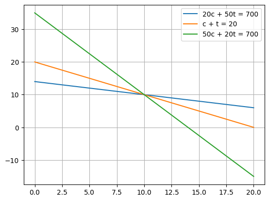
Example: An overdetermined, consistent linear system (our headscratcher from the early lectures!)

\(20 c + 50 t = 700\)

\( c+t = 20\)

\( 50 c + 20 t = 700\)

which gives the linear system:

\[\begin{split}\begin{bmatrix} 20 & 50 \\ 1 & 1 \\ 50 & 20 \end{bmatrix} \begin{bmatrix} c \\ t \end{bmatrix} = \begin{bmatrix} 700 \\ 20 \\ 700 \end{bmatrix} \end{split}\]

#Plot it!

import matplotlib.pyplot as plt
import numpy as np

# Define the x values
x = np.linspace(0, 20, 100)

# Calculate the y values for the first equation (20c + 50t = 700)
y1 = (700 - 20 * x) / 50

# Calculate the y values for the second equation (c + t = 20)
y2 = 20 - x

# Calculate the y values for the third equation (50c + 20t = 700)
y3 = (700 - 50 * x) / 20

# Plot the lines
plt.plot(x, y1, label='20c + 50t = 700')
plt.plot(x, y2, label='c + t = 20')
plt.plot(x, y3, label='50c + 20t = 700')

# Add a grid
plt.grid(True)
plt.legend()
plt.show()

#The arrays are:
# ~~ Question - what is the linear system and how do we solve it?

A = np.array([[20, 50], [1, 1], [50, 20]])
b = np.array([700, 20, 700])

#x = np.linalg.solve(A, b)

M = np.linalg.inv(A.T @ A)@A.T
print(np.linalg.pinv(A))
print(M-np.linalg.pinv(A))
print(M@b)





# ~~ Answer
# A = np.array([[20, 50], [1, 1], [50, 20]])
# b = np.array([700, 20, 700])

# #x = np.linalg.solve(A, b)

# M = np.linalg.inv(A.T @ A)@A.T
# print(M)
# print(np.linalg.pinv(A))
# print(M-np.linalg.pinv(A))
# print(M@b)

[[-0.00952672  0.000204    0.02380661]
 [ 0.02380661  0.000204   -0.00952672]]
[[-1.73472348e-18  2.71050543e-19  6.93889390e-18]
 [ 1.04083409e-17 -3.25260652e-19 -1.73472348e-18]]
[10. 10.]

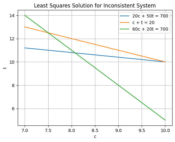
Example: An overdetermined, inconsistent linear system

\(20 c + 50 t = 700\)

\( c+t = 20\)

\( 60 c + 20 t = 700\)

import matplotlib.pyplot as plt
import numpy as np

# Define the x values
x = np.linspace(7, 10, 100)

# Calculate the y values for the first equation (20c + 50t = 700)
y1 = (700 - 20 * x) / 50

# Calculate the y values for the second equation (c + t = 20)
y2 = 20 - x

# Calculate the y values for the third equation (60c + 20t = 700)
y3 = (700 - 60 * x) / 20

# Plot the lines
plt.plot(x, y1, label='20c + 50t = 700')
plt.plot(x, y2, label='c + t = 20')
plt.plot(x, y3, label='60c + 20t = 700')

plt.xlabel('c')
plt.ylabel('t')
plt.title('Least Squares Solution for Inconsistent System')
plt.legend()
plt.grid(True)
plt.show()

Where do you think he solution is going to be?

A = np.array([[20, 50], [1, 1], [60, 20]])
b = np.array([700, 20, 700])

#np.linalg.(A, b)
x_lsq = np.linalg.pinv(A)@b
print(x_lsq)
x_lsq,_,_,_ = np.linalg.lstsq(A,b)
print(x_lsq)

# Plot the lines
plt.plot(x, y1, label='20c + 50t = 700')
plt.plot(x, y2, label='c + t = 20')
plt.plot(x, y3, label='60c + 20t = 700')


plt.plot(x_lsq[0], x_lsq[1], 'ro', label='Least Squares Solution')
plt.xlabel('c')
plt.ylabel('t')
plt.title('Least Squares Solution for Inconsistent System')
plt.legend()
plt.grid(True)
plt.show()

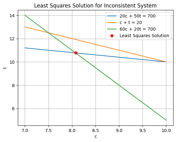
[ 8.07704251 10.76953789]
[ 8.07704251 10.76953789]

<ipython-input-7-52bb65e377be>:7: FutureWarning: `rcond` parameter will change to the default of machine precision times ``max(M, N)`` where M and N are the input matrix dimensions.
To use the future default and silence this warning we advise to pass `rcond=None`, to keep using the old, explicitly pass `rcond=-1`.
  x_lsq,_,_,_ = np.linalg.lstsq(A,b)

Was this what you were expecting?

Weights

As with most approximate methods, the moment we start to move away from an exact solution subtle effects start to show up!

Notice we are minimizing the residuals but there is a subtle problem with the problem definition above:

\[\begin{split}\begin{align} 20 c + 50 t &= 700 \\ c+t &= 20 \\ 60 c + 20 t &= 700 \end{align} \end{split}\]

The coefficients of the second equation is about an order of magnitude lower than the others. Of course this system is equivilant to:

\[\begin{split}\begin{align} 20 c + 50 t &= 700 \\ 10c+10t &= 200 \\ 60 c + 20 t &= 700 \end{align} \end{split}\]

or even

\[\begin{split}\begin{align} 0.2 c + 0.5 t &= 7 \\ c+t &= 20 \\ 0.6 c + 0.2 t &= 7 \end{align} \end{split}\]

What does this remind you of?

Jacobi (diagonal) preconditioning!

\[\begin{split}P^{-1} = \begin{bmatrix} W_{1} & 0 & 0 \\ 0 & W_{2} & 0 \\ 0 & 0 & W_{3} \end{bmatrix} \end{split}\]

If we define \(r_1, r_2, r_3\):

\[\begin{split}\begin{align} 20 c + 50 t -700 &= r_1 \\ c+t -20 &= r_2 \\ 60 c + 20 t -700 &= r_3 \end{align} \end{split}\]

We say the residuals are / can be weighted, i.e.: the least squares problem becomes,

\[ Min_x \ of \ \sum W_i^2 r_i \]

Let’s code it!

A = np.array([[20, 50], [1, 1], [60, 20]])
b = np.array([700, 20, 700])

#~~ Question: What's the preconditioner? How do we apply it?
Pi = np.diag([1,7,1])
print(Pi)
A = Pi@A
b = Pi@b
###

#~~ Answer
# Pi = np.diag([1,70,1])
# print(Pi)
# A = Pi@A
# b = Pi@b
###



x_lsq,_,_,_ = np.linalg.lstsq(A,b)

print(x_lsq)

# Plot the lines
plt.plot(x, y1, label='20c + 50t = 700')
plt.plot(x, y2, label='c + t = 20')
plt.plot(x, y3, label='60c + 20t = 700')


plt.plot(x_lsq[0], x_lsq[1], 'ro', label='Least Squares Solution')
plt.xlabel('c')
plt.ylabel('t')
plt.title('Least Squares Solution for Inconsistent System')
plt.legend()
plt.grid(True)
plt.show()

[[1 0 0]
 [0 7 0]
 [0 0 1]]
[ 8.08267345 10.78401744]

<ipython-input-13-2aa1c6412f60>:20: FutureWarning: `rcond` parameter will change to the default of machine precision times ``max(M, N)`` where M and N are the input matrix dimensions.
To use the future default and silence this warning we advise to pass `rcond=None`, to keep using the old, explicitly pass `rcond=-1`.
  x_lsq,_,_,_ = np.linalg.lstsq(A,b)

Weights are an excellent way to introduce measurement uncertainty into your fit!