Motivating example

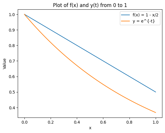
Consider an ODE \( y^\prime = -y \quad y(0) = 1\), which has an analytical answer \(y = e^{-t}\).

We wish to approximate this function numerically between \([0,1]\) with a line defined by the boundary points, \(f(0) = a = 1\) and \(f(1) = b\), $\(f(x) = [1-x] + x b\)$

How do we find \(b\)?

Option 1: Direct substitution

Following the Finite Difference method, we can subsitute \(f(1)\) into the ODE and solve for b:

\[\begin{split}\begin{align} f'(1) &= f(1) \\ b-1 &= -b \\ b &= 1/2 \end{align}\end{split}\]

and the approximate solution is \(f = 1 -\frac{x}{2}\)

import numpy as np
import matplotlib.pyplot as plt

# Define the functions
f = lambda x: 1 - x / 2
y = lambda t: np.exp(-t)

# Generate values
x = np.linspace(0, 1, 100)
f_values = f(x)
y_values = y(x)

# Plot the functions
plt.plot(x, f_values, label='f(x) = 1 - x/2')
plt.plot(x, y_values, label='y = e^{-t}')
plt.xlabel('x')
plt.ylabel('Value')
plt.legend()
plt.title('Plot of f(x) and y(t) from 0 to 1')
plt.show()

Option 2: Least square minimization of the residual

Let’s integrate the squared residual of f(x) plugged into the ODE, \(y^\prime + y\)

\[\begin{split}\begin{align} R &= f^\prime(x) +f(x) \\ &= [b-1] + 1-x + x b \\ &= b+x[b-1] \\ R^2 &= b^2 + 2 b x[b - 1] + [x[b - 1]]^2 \\ F = \int_0^1 R^2 \ dx &= \frac{1}{3} [7 b^2 - 5 b + 1] \\ \end{align} \end{split}\]

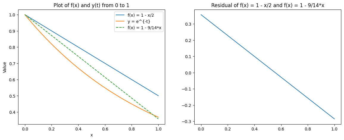
Note that in the end the integral of the residual, \(F\) is a parabolic function of the parameter \(b\). The minimum is found at: \(\frac{\partial F}{\partial b}(b) = 0\), for \(b = \frac{5}{14}\). The approximate solution is \(f(x) = 1-\frac{9}{14}x\).

# Define the new function
fig, axs = plt.subplots(1, 2, figsize=(14, 5))
f_new = lambda x: 1 - 9./14*x
f_new_values = f_new(x)


# Plot the functions
axs[0].plot(x, f_values, label='f(x) = 1 - x/2')
axs[0].plot(x, y_values, label='y = e^{-t}')
axs[0].plot(x, f_new_values, label='f(x) = 1 - 9/14*x', linestyle='--')
axs[0].set_xlabel('x')
axs[0].set_ylabel('Value')
axs[0].legend()
axs[0].set_title('Plot of f(x) and y(t) from 0 to 1')

# Plot the residual
residual = lambda x: -9/14 + 1 - 9./14*x
axs[1].plot(x, residual(x))
axs[1].set_title('Residual of f(x) = 1 - x/2 and f(x) = 1 - 9/14*x')

plt.show()

We see that option 2 does a better job of approximating the function over the full domain since it focusses on the integral of the residual.

You may have noticed that we did something funny here: we integrated \(R^2\) and then took its derivative with respect to \(b\) in order to find the minimum of the integral! I.e.:

\[\begin{split}\begin{align} \frac{\partial F}{\partial b} = 0 &= \frac{\partial }{\partial b} \int_0^1 R^2 \ dx \\ &= \int_0^1 2R \frac{\partial R}{\partial b} \ dx \\ &= \int_0^1 R v \ dx \end{align} \end{split}\]

where the residual has now been weighted by the function \(v\). This is called the Method of Weighted Residual [MWR]. Let’s try a different function and see what happens.

Option 3: Integrate the MWR to find the parameters

Integrate the weighted residual function directly with a convenient choice of \(v\).

lets take \(v = x\) (to be motivated later) and integrate:

\[\begin{split}\begin{align} \frac{\partial F}{\partial b} =0 &= \int_0^1 R x \ dx \\ &= \int_0^1 \big[b+[b-1]x\big]x \ dx \\ &= \int_0^1 b x+[b-1]x^2 \ dx \\ &= \bigg[ \frac{1}{6} x^2\big[3b+2[b-1]x\big]\bigg]_0^1 \\ &= b-\frac{2}{5} \\ \end{align} \end{split}\]

which is very close to our previous solution \(b = \frac{5}{14}\) but with a simpler integration. BUT, we are still let with analytically integrating! If only there were a way to express integrals as the sum of the integrand evaluated at certain points…

Option 4: Express the MWR integral as the sum of the integrand evaluated at certain points.

Integrate the weighted residual function directly with a convenient choice of \(v\) as the sum of the integrand evaluated at certain points:

Recall Gaussian Quadrature allows us to evaluate an integral by summing the integrand at the Gauss Points. The Gauss Points for the domain \([-1,1]\) are \(\pm\frac{1}{\sqrt{3}}\), scaled to this integral domain become,

\[\begin{split} \begin{align} x_{[0,1]]} &= 0.5 (x_{[-1,1]} + 1) \\ &= \frac{1}{2} \bigg[1 \pm\frac{1}{\sqrt{3}} \bigg] \\ &\approx [0.21132487, 0.78867513] \end{align} \end{split}\]

and

\[\begin{split}\begin{align} 0 &= \int_0^1 R x \ dx \\ &= Rx (x=.21132487) + Rx(x = .78867513) \\ &= -0.0446582 + 0.255983 b -0.622008 + 1.41068 b \\ b &= \frac{2}{5} \end{align} \end{split}\]

Recap of the approach

Let’s recap what we’ve done:

1. parameterized a function as a weighted sum of simpler functions (a linear basis)

2. found a (simple) integral expression that minimizes the error in the approxiation (Minimized Weighted Residual)

3. performed the integration exactly using only function evaluations into a linear system (Gaussian quadrature)

4. Solved the linear system (I told you everything boiled down to linear systems!)

Practical solution of linear systems requires sparsity! Let’s formalize our proceedure and see how we can ensure sparsity.