Conditioning

The matrix interpretation is troubling. The solvability of these systems is related to \(det(A)\) and we have 2 data points:

1. \(|A| = -30\) and the system is solvable.

2. \(|A| = 0\) and the system is unsolvable.

What is the significance of \(-30\)?. What happens when \(|A| \rightarrow 0\) ?

We saw \(|A| \rightarrow 0\) when we adjusted the price of tables. Let’s play with that! Set the cost of tables to \(20-\epsilon\).

\(|A| = 20-20+\epsilon = \epsilon\)

Now look at the inverse equation:

\(A^{-1} \sim \frac{1}{|A|} \sim \frac{1}{\epsilon}\)

As \(\epsilon →0\), this fraction goes to infinity!

The problem is:

\(20 c + [20+\epsilon] t = 700\)

\( c + t = 10\)

Graphically,

import matplotlib.pyplot as plt
import numpy as np

# Define the x values
x = np.linspace(-200, 30, 100)

# Define the epsilon values
epsilons = [0, -1, -10, -30]

plt.plot(x, 20 - x, label='c + t = 20', linewidth = 3)

# Plot the lines for each epsilon value
for epsilon in epsilons:
  y1 = (700 - 20* x) / (20 - epsilon)

  # Plot the lines
  plt.plot(x, y1, label=f'epsilon = {epsilon}')

# Add labels and title
plt.xlabel('Number of Chairs (c)')
plt.ylabel('Number of Tables (t)')
plt.title('Fundraising Event with Varying Epsilon')

# Add a grid
plt.grid(True)

# Add a legend
plt.legend()

# Display the plot
plt.show()

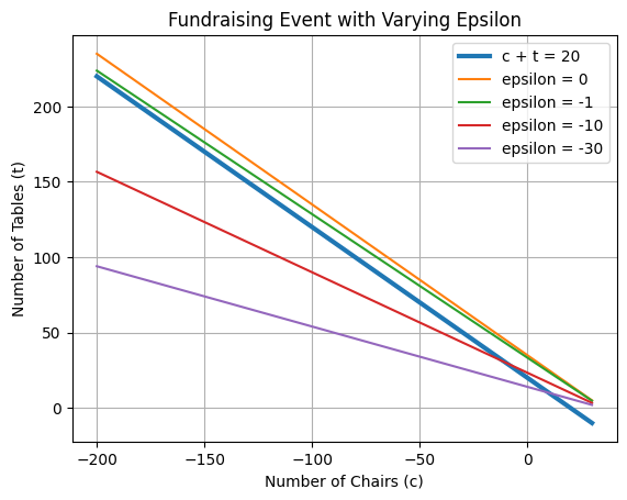
The lines are getting more and more parallel / linearly dependent.

NOTE: There is a solution until \(\epsilon =0\), but the answer is both moving away and moving at an increasing rate!

Elimination

Let’s use \(c = 20-t\) and substitute into the first equation:

\( 20 [20 -t] + [20-\epsilon] t = 700\)

\(\epsilon t= 300\)

\( t = 300 / \epsilon\)

and again we see an infinite answer.

Ex:

\(\epsilon\)	t	c
-30	10	10
-10	30	-10
-1	300	-280
0.1	3000	-2980
1e-20	3e+22	-3e+22
0	\(\infty\)	\(-\infty\)

This should sound alarm bells!

1. Recall roundoff error - 1e-20 is well within the range of roundoff error. Here, even just recording the matrix element value can cause astronomical changes in the solution!

2. These coefficients typically have some uncertainty which compounds the numberical uncertainty.

The condition number

Let’s try to quantify this issue by returning to the importance of \(|A| = -30\). We could multiply the first equation by an arbitrary scalar § and the determinant would scale accordingly, so obviously the magnitude of \(|A|\) can’t be important.

It is only important relative to the magnitude of the equation coefficients (the elements of \(A\)).

Matrix norms

For vectors we know the magnitude (called the norm) is: \(||v|| = \sqrt{\sum_n v_i^2} = \sqrt{v\cdot v}\).

In fact this is more than one type of vector norm. In general, \(||v||_p = \sum_i \left(v_i^p\right) ^{1/p}\). The p=2 norm is the ‘Euclidian norm’, for \(p\rightarrow \infty\), \(|v|_{\infty} = max(v_i)\).

The Euclidian / Frobenius norm is simply,

\(||A||_F = \sqrt{\sum_{i=1}^{m} \sum_{j=1}^{n} |A_{ij}|^2}\)

\(||A||_F = \sqrt{A:A}\)

Infinity Norm (maximum row-sum norm)

\(||A||_\infty = \max_{1 \le i \le m} \sum_{j=1}^{n} |A_{ij}|\)

Spectral, or 2-norm \(||A||_2 = \max(eigen value)\)

The determinant is considered small in comparison with the matrix norm \(|A| << ||A||\).

In actuality, C.N. = \(\frac{max(eigenvalue)}{min(eigenvalue)}\) but hard to find.

The matrix condition number

\(cond(A) = ||A|| ||A^{-1}||\)

is the formal measure of conditioning. For \(cond(A) ~1\) the matrix is well-conditioned and its inversion is numerically stable. Otherwise it is ill-conditioned and we will need to do something else.

If the eigenvalues can be calculated (or estimated) then we can do the spectral condition number,

\(cond(A) = \frac{\max(e.v.)}{\min(e.v.)}\)

(generallized to singular values).

BONUS head-scratchers!

Lets go back to the original problem

(1) \(20 c + 50 t = 700\)

(2) \( c+t = 20\)

and add some other requirement that amounts to:

(3) \( 50 c + 20 t = 700\)

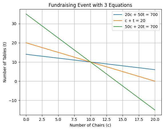
Some quick math will show these lines are linearly independant, and graphically we see there is a solution,

# prompt: Plot the 3 lines above

import matplotlib.pyplot as plt
import numpy as np

# Define the x values
x = np.linspace(0, 20, 100)

# Calculate the y values for the first equation (20c + 50t = 700)
y1 = (700 - 20 * x) / 50

# Calculate the y values for the second equation (c + t = 20)
y2 = 20 - x

# Calculate the y values for the third equation (50c + 20t = 700)
y3 = (700 - 50 * x) / 20

# Plot the lines
plt.plot(x, y1, label='20c + 50t = 700')
plt.plot(x, y2, label='c + t = 20')
plt.plot(x, y3, label='50c + 20t = 700')

# Add labels and title
plt.xlabel('Number of Chairs (c)')
plt.ylabel('Number of Tables (t)')
plt.title('Fundraising Event with 3 Equations')

# Add a grid
plt.grid(True)

# Add a legend
plt.legend()

# Display the plot
plt.show()

so what do we do now?!? (Attend advanced numerical methods to learn about pseudoinverses!)